Who Are Your Trainers Neighbors

Tags

tweet

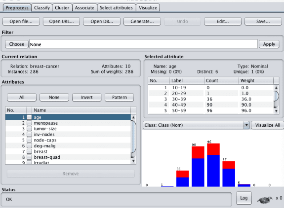
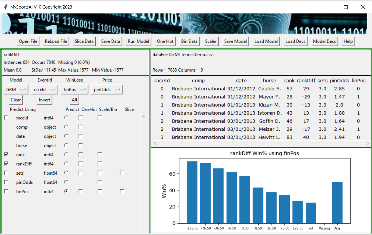
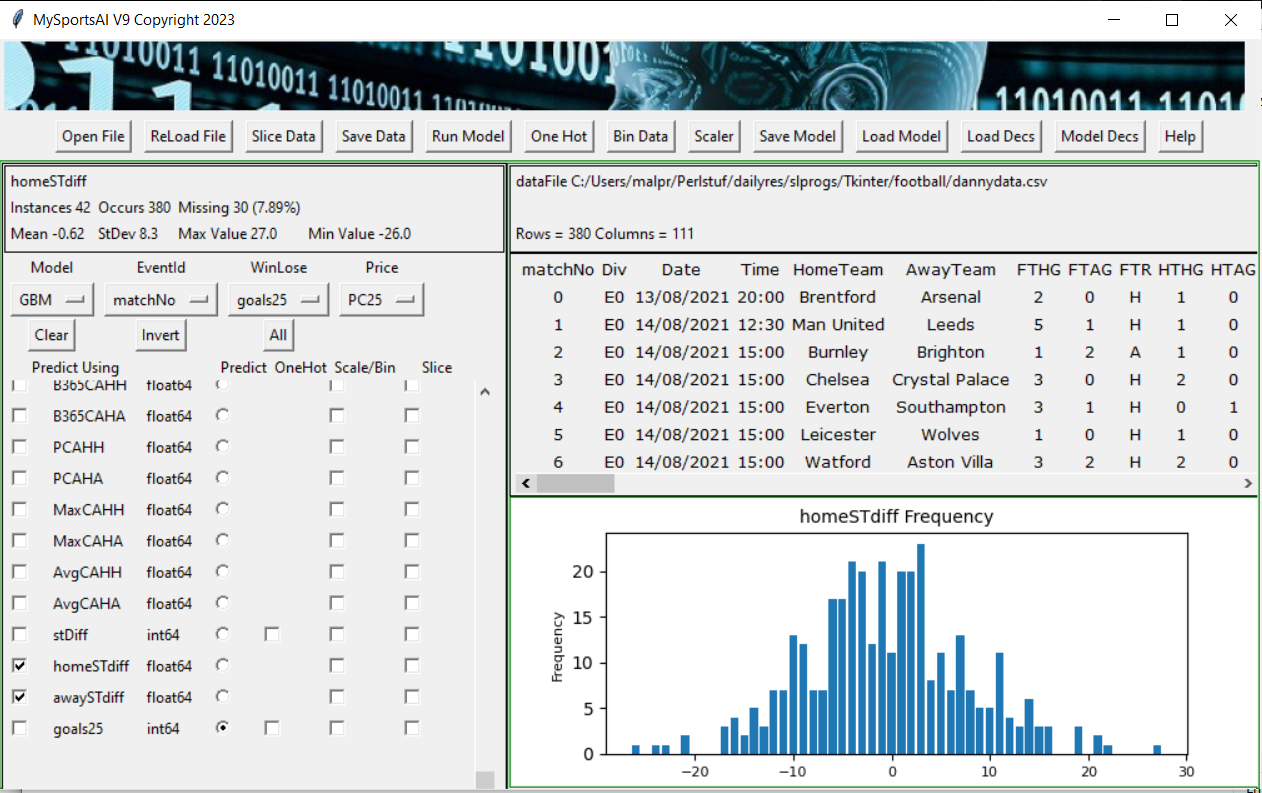
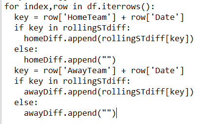
What should we be looking at with regard to trainers in lets say a class 5 or 6 handicap horse race. Current trainer form ?, jockey booking ?, course record ?. Different pundits have different preferences but usually current form figures strongly. One possible problem with this is that we are lumping all trainers together. Trainers most likely have a different pecking order of influences that effect their winning ability. Using MySportsAI you can check the correlation of an array of factors for a given trainer but on this occassion I decided to write some Python code to go through all the features in MySportsAI and order them in terms of correlation to winning for each trainer with more than 500 runs from 2011 to 2019.

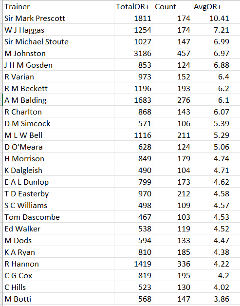
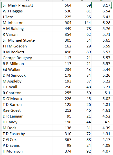
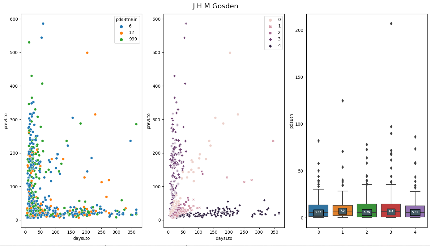
Let’s look at a specific example before getting carried away with models. The vast majority of trainers have a negative correlation between days since last run and winning. This correlation varies in size but a few have a positive correlation. M Johnston (now retired is one). It is not his strongest feature but he does buck the trend.

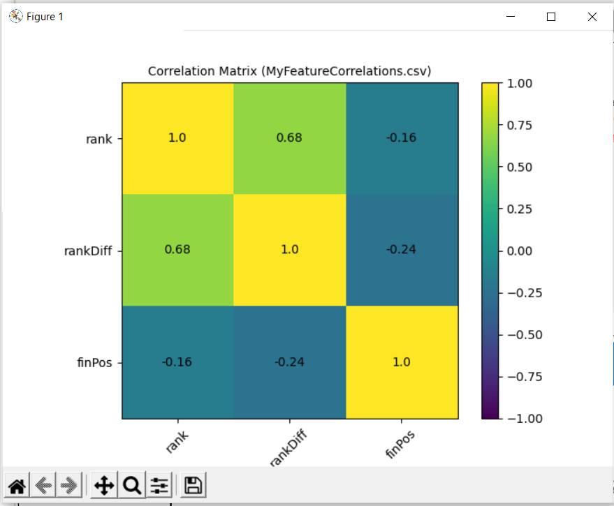
I identified that the top 4 correlated features for R A Fahey, they are runnerRatio hasPlacedTrack beatLto1 logPrevBFSP

Things are not the same for Karl Burke, he has the same top ranked feature but in second is the average track win pace (I would have to dig further to find out why) and in third is whether the horse has placed at the track

The idea I am leading to is whether individual models based on the relevant features for each trainer could lead to a more precise ability to detect when a trainer is most likely to win. Of course if the market accounts for this we may be up a cul de sac but we will not know until test the idea.

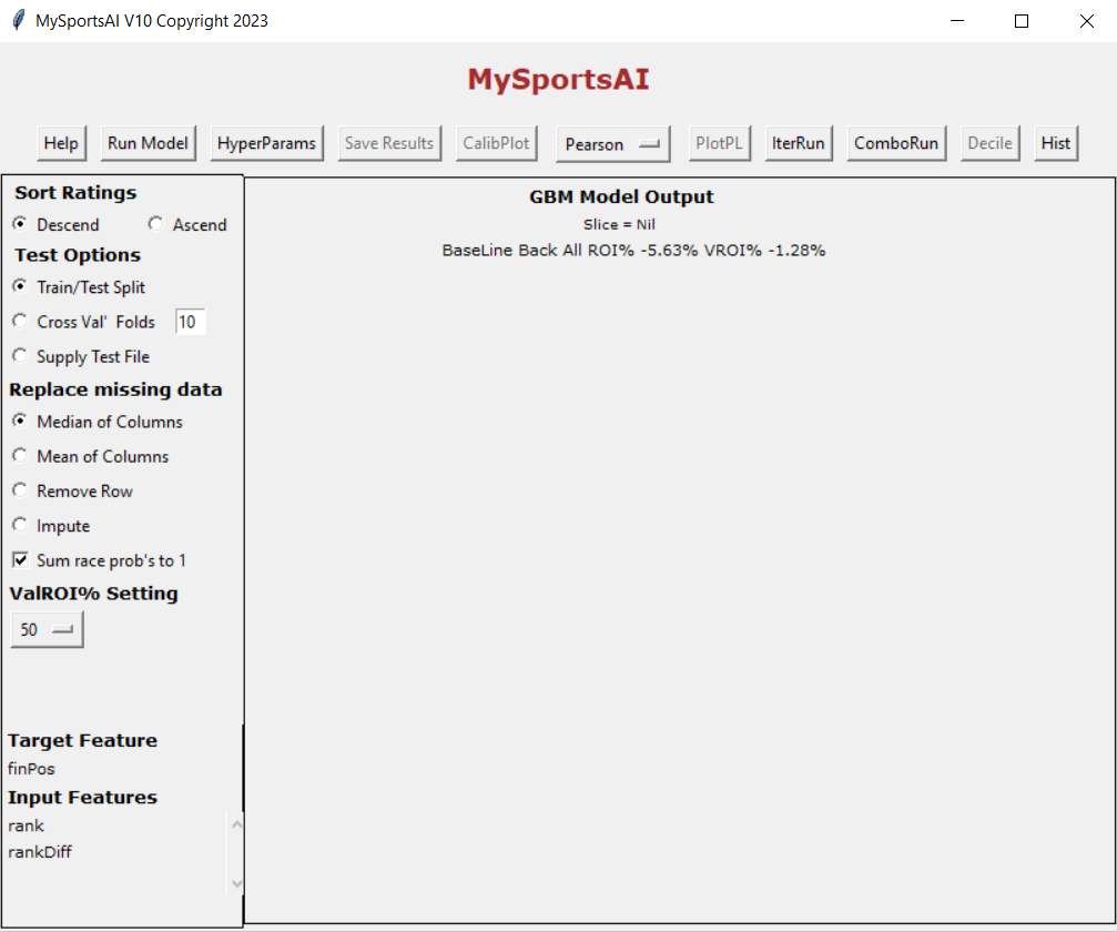
My first port of call was to create models for each trainer based on the top (in terms of correlation to winning) X features for each trainer. The next step was to see if the predicted probabilities for races the trainer had runners in within the test set (in this case 2021 to 2023) performed better when they were greater than the trainers base win rate. I focused the attention down to handicaps of class 5,6 and 7. I think class has an impact on how horses are prepared and hence the correlation of features. I started with K Nearest Neighbor algorithm for the model taking care to normalise all features that were used in the models. Here are the results for various number of top ranked features, that is to say using only the top feature for each trainer and then the top 2, top 3 etc. All profit/loss is to Betfair SP minus 2% commission

Using top 1 feature and probability greater than trainer base strike rate

Bets 10,126 Variable PL +7.64 Variable ROI% 0.43%

Using 1 feature and probability less than base strike rate

Bets 25,272 VPL -103.66 VROI% -3.15%

Using top 2 features and probability greater than base strike rate

Bets 8,856 VPL -12.92 VROI% -0.87%

Using top 2 features and probability less than base strike rate

Bets 25,028 VPL -105.68 VROI% -3.14%

Using top 3 features and probability greater than base strike rate

Bets 10,661 VPL -58.2 VROI% -3.05%

Using top 3 features and probability less than base strike rate

21,913 VPL -68.3 VROI% -2.47%

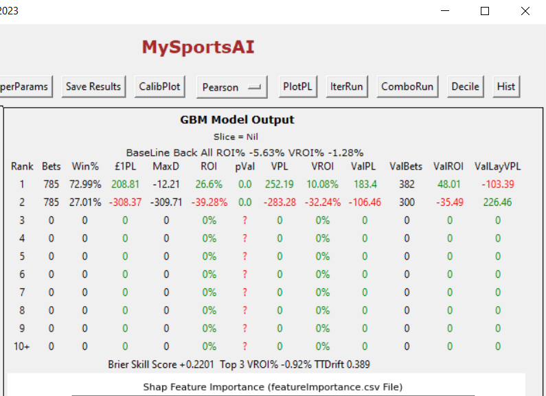
Four features continued the trend and so it seems that less is more in this case. The generation of a small profit is encouraging. A next step may be to investigate different model algorithms. A quick look at a GBM produced.

Using top 1 feature and probability greater than trainer base strike rate

Bets 11,431 Variable PL -26.8 Variable ROI% -1.43%

A Logistic Regression model produced

Using top 1 feature and probability greater than trainer base strike rate

Bets 10,762 Variable PL +16.96 Variable ROI% +0.89%

Improving 3yos By Trainers

Tags

tweet

The start of a new flat season is only a couple of weeks away and a host of lightly raced or unraced 3yo’s will be trying to make a name for themselves. I took a look at how trainers perform in terms of improving their lightly raced 3yo’s. To do this I checked all trainers for the last 14 years, logging their 3yo runners initial official rating when having traced less than 5 times. I then logged each horses best OR rating achieved throughout a given year if they did not switch trainers. To avoid horses having just one run after getting their OR and then perhaps being injured I ensured all horse in the sample had run at least 6 times. This exercise gave a total positive or negative value of overall OR gain for each trainer from which I then calculated an average OR gain to see who on average makes the greatest strides with lightly raced 3yo’s.

No prize for guessing who comes out top. Here is a breakdown showing only trainers who have had at least 100 runners.

Looking now at fillies where trainers have had at least 20 runners and generally we see less improvement although one or two ‘lesser’ trainers get a mention, J Tate in particular.

You have to wonder why more trainers do not apply Prescott’s aggressive form of handicapping in order to gain the best advantage for their owners. Looking at J Tates 3yo fillies he has the following 2023 2yo fillies potentially running this year as 3yo’s

Invincible Tiger

Talent Show

Belle Storm

Ahlain

Lumiere D’or

Garden View

Qamari

Have an enjoyable and profitable 2024 flat season

Is PRIM the Proper Way to Develop Systems

Tags

ai, artificial-intelligence, data-science, Machine Learning, python, tweet

First up a thank you to my friend Steve Tilley for pointing me towards PRIM, I must admit I had not heard of it until he tweeted me. PRIM stands for Patient Rule Induction Method, so what has it got to do with building race betting systems. If you have had a go at building a system you are familiar with being faced with an array of variables to choose from. Examples of these would be days since the horse last ran, is it a course and/or distance winner and so on. Picking the right combination is one part of the task but also picking the subset of each variable is an additional task. For example are you better off picking horses that ran between 10 an 15 days or is 15 to 30 the sweet spot.

The algorithm for PRIM revolves around ‘Peeling’ and ‘Pasting’. I am going to focus on Peeling which essentially involves shrinking the entire data set gradually. Each step of shrinkage involves removing a subset of rows of data starting with the most ‘worthy’ subset. Of course ‘worthy’ means different things to different applications but with the algorithm you can specify what value of worhtiness to rank the subsets on.

Let me be a bit more specific. Take days since last ran. I am going to have my test of worthiness coded as variable profit or loss, so in other words profit when attempting to gain £1 at the odds on each bet. The algorithm will now search the data space on days since last ran using small incremental steps (which we can specify) until it finds the optimum in terms of (in our case) profit. Let us imagine it finds the most profitable to be between 2 and 6 days, it will then remove this subset of data from the overall data and then repeat the process in order to find the second best fit and so on.

It is possible therefore to use PRIM to find the first best fit on a series of data variables of interest, which variables you may ask. I would suggest bearing in mind that consistency of distribution in terms of profit is important. A variable that has wild swings may be less easy to tolerate even if overall more profitable than a lesser variable that is consistent say across years.

I applied PRIM to the following variables from MySportsAI data for 2011 to 2016 for Handicaps

[‘daysLto’,’prevLto’,’TRSR’,’TRinrace’,’avgBeat’,’runnersRatio’,’pdsBtnLto’,’daySinceGR’,’Jockinrace’,’SireSurf’,’IPDropPercent’]

I then took the top located segment form the top 2 ranked based on the reported mean measure from PRIM (Note not sure at this stage what the means measure is but it go’s gradually down for each variable as it reports the top down to bottom located segments). Using this as a system applied to 2016/17 produced the following.

Just using the top ranked variable daysSinceGR (days since good run) produced

980 bets PL after comm +26.1 to BFSP

Now using the top two variable segments applied together produced

119 bets PL + 9.43

Note to readers – after some Twitter user baulked at the profit on one of my articles. Articles like this are more about informing the reader of a method or a piece of software, the PL is just a final line of information. It is intended to spark the readers interest not deliver on a plate a winning system. As I often say to people, reading Nick Mordin when he used to publish weekly was not really about finding a golden goose but more about being influenced by a way of thinking. The most valuable things I have learnt over the years have been about thinking and not a specific winning strategy.

You can find out more about PRIM from this article

https://towardsdatascience.com/find-unusual-segments-in-your-data-with-subgroup-discovery-2661a586e60c#

Please do not forget to rate the article and feedback is welcome in the comment

A Blast From The Past

Tags

tweet

I was rummaging through some of my old SmartSig mags the other day along with email exchanges from the old SmartSig email forum. It was nice to conjur up some of those old names from the early noughties. One email caught my eye and seemed equally relevant today so I thought I would reproduce it here verbatim from 2005.

A couple of thoughts (as a practicing statistician) on your approach.

The process of selecting the best variable, then the next bet variable to pair up with the first etc etc can lead you to a local best fit rather than a global bets fit. In other words you end up finding the best fit given that you say chose age as your first variable when in fact a better fit exists if you chose jockey strike rate first (even though age was a better predictor than jockey strike rate on its own).

For this reason it would be better to search all possible combinations rather than sequentially adding the next best variable. Of course this will add significantly to the computing time required !.

Also I feel that equal weighting of variable will reduce your fit (and consequently forecasting ability) quite significantly. The impact will depend on your variables and how they are calculated but will be exacerbated if you have variables with widely different means and standard deviations.

For instance of you have position last time out as a factor (taking values 1,2,3 up to say 20). Official ratings from typically 80 to 140 and forecast SP from 0.2 to 200, then giving equal weight to each (ie adding them together to produce a rating) would have a significant impact on your fit and whether a variable was included as each variable has its own very different impact on the subsequent rating. Variable weights are vital to effectively scale the input variable to match what you are predicting.

To get round this I convert each of my factors to strike rate so that everything has a range of 0 to 100 (ie historical strike rate of horses finishing 1st last time out, 2nd last time out etc). For variables like official rating the historical samples become too low to accurately calculate each point so I calculate in groups (bins) (eg 70 to 79, 80 – 89 etc). The fit a line to the groups to give me a decent interpolation in between groups.

Even then the adjusted variables need variable weights to produce the rating because they have different ranges. For instance Jockey strike rate over the last 14 days would be quite variable (0 – 100) whereas trainer strike rate over the last 12 months would be more stable (5-25). Jockey strike rate might not get into your model because those cases where it was 100 (big increase in rating) did not result in a big increase in strike rate (or whatever you are trying to predict). However, weight jockey strike rate by say 0.1 (range is now 0 to 10) and it may now start to more closely reflect the variable you are tring to predict and hence get into your model.

(Of course the input variables may not be linear in their impact – ie jockey strike rate may be important up to say 25% but anything in the range 26% to 100% adds nothing extra – but that is a whole new set of complications)

Most statistical modelling techniques (typically regression of some sort) derive from the need to find a set of weights that give you the global best fit. so overcoming both the above issues. The techniques are elegant in that sense and were developed at a time when computers did not exist and it was impossible to crunch through 1000’s of alternatives.

Putting your database through a regression fo some sort would, I feel save you a lot of time and guarantee the best possible fit. It is effectively a short cut through the number crunching you are doing with a guarantee of finding the best possible answers.

A couple of other things I have learnt in generating my own ratings.

My aim is profit but in developing ratings I felt I had to focus on strike rate for reasons other people have discussed. (ie focus on LSP and the model will seriously be effected by one or two 100/1 winners). By focusing on strike rate your prediction of horses coming 2nd, 3rd etc should improve.

I specifically ;eave out forecast SP even though this is the best single factor for predicting strike rate – simply because this reflects the crowd and in trying to find an edge it is better not to follow the crowd.

I find it is also important to include a way of filtering out extremes and dealing with missing values. eg a jockey who has won 1 from 1 so has a 100% strike rate may need pulling back to 25%.

In this respect there is nothing better than looking at graphs/charts/tables of all your variables to examine what is extreme and whether there are any non linear elements to them.

Many thanks to Paul Dyson for this post

What’s My Name

Tags

tweet

Kinky handicapping is a USA term used to describe bet selection methods that involve obscure or unusual paths. A book called Kinky Handicapping was published which I think is now out of print. Certainly a few years ago when I tired to get a copy it was out of print.

In a recent exchange with @FlatStats on Twitter things got kinky, we discussed briefly the possibility that punters under or over bet certain names. Steve Tilley replied and described it as the Willie Wumpkins effect. What he meant was the idea that perhaps punters are more likely to over bet Bringhomethebacon and under bet Rogue Thunder in the 5.30 at Chelmsford tonight. Does the tone of or sentiment of a horse name pull the prices one way or another.

I mentioned that a branch of Machine Learning called Sentiment Analysis might be able to help with analyzing this problem. Sentiment analysis can take a block of text eg a book review and decide on a scale of 1 to 10 how positive or negative it is. The same thing could be done for horse names especially if your trained the model in terms of price drifting or dropping.

I wanted to look into this but was pressed for time with other projects so I decided to do a quick cut down examination to satisfy my curiosity and what I came up with surprised me.

First of all I gathered together the 100 most popular English male and female names giving a total of 200 names. I then analysed race results for both codes to see if horse names that contained human names were overbet. I started off analysing 2010 to 2014 which produced a surprising result.

20,617 bets producing to variable stakes (ie to always win £1) stakes = 3143 PL = + 28.14 ROI +0.89%

One could be forgiven for thinking this subset may be a platform for further pruning and higher profit. The horse which did not contain a name produced.

431,620 bets and Variable ROI of -1.82%

So far so good, let us now take a look at 2015 to 2018

16,810 bets Variable ROI = +1.62%

We now have over 37,000 bets and a profit to work from. Finally let us take a look at 2019 to 2022

15,127 bets variable ROI = -5.17%

Bloody hell the wheels well and truly fell off, during that period you would have lost 114 points to variable stakes. So if you were backing to win £1 you would have lost £114. Over the whole period the results are as follows

52,603 bets varPL = -43.9 ROI = -0.55%

The surprise here is that you lose less backing horses that contain English names, but the latter period would have been difficult to wade through. One caveat to this is that I did not separate those where the name was embedded, for example if Greg was in the list of popular names then a horse called Gregorina would be flagged. This could be a worthy avenue of further investigation but I think overall it suggests that names are not entirely neutral and when I get round to it a further blog post utilising sentiment analysis could be interesting. Kinky handicapping lives on.

Tennis Modelling with MySportsAI

Tags

tweet

I had an interesting exchange on Twitter yesterday with a top Tennis tipster who asked me whether it would be feasible for him to get involved in coding and Machine Learning in order to explore ML and Tennis modelling. The answer is of course yes but if you are starting from scratch there is a steep learning curve and you will have to invest time.

I advised him that their are non coding alternatives. For example you can explore ML models through the GUI interface that comes with WEKA

WEKA however does not provide profit and loss analysis which of course is important when we are building betting models. I suggested he try MySportsAI but it became clear to me that describing how to use MySportsAI for tennis modelling when it is primarily created for horse racing was a little difficult via Twitter messaging. In this blog I am going to demo how to lay out data and build a very simple model using Tennis data. It is not a profitable model, created only for demo purposes.

OK here is a screen shot of MySportsAI loaded up with some basic Tennis data

You will notice that the first 7 lines of this 7888 line data file are displayed on the upper right side. The first thin =g to notice is that the data has 2 lines per match. The other thing to notice is that I have labelled some of the columns rather oddly. For example the match ID is actually called raceId and the players are called horse. This is to allow MySportsAI to make sense of the columns or identify the columns when it outputs its results. I may make some changes to MySportsAI in future to alleviate this oddity but for now its a minor distraction, nothing more.

On the left we can see that there are 3 columns that we may want to use as inuts to our model namely rank, rankDiff and sets. For Tennis fans these terms should be obvious but if you are new to Tennis Giraldo is ranked 57 and Mayer 28. The rankDiff column is simply the rank difference of a player to his opponent.

pinOdds are the pinnacle closing line odds for the players and the finPos column designates with a 1 or a 0 who won the match. To the upper left I have made sure finPos and pinOdds are designated as the WinLose and Price features to be used by the model

There are a number of ML algorithms to choose from in the drop down list but I have chosen GBM.

Putting the cursor over a feature name or type will show on the lower right the frequency distribution or the win distribution respectively.

OK let us click ‘Run Model’ using rank and rankDiff as input features to produce the following window

The train/test window appears. I have not yet created any results or a model even but first I need to set certain parameters. I am telling MySportsAI to organise the ratings it produces in descending order. We are going to perform a train/test split which simply means train the model on 80% of the data and then test the model it creates on the remaining 20%. I am also telling it to replace any missing data with the median of the column it resides in and finally sum the probabilities it produces to 1 for a given match.

After clicking ‘run model’ in this window we get

We can see that the top rated player in each match made a loss of -23.15 whereas the second top lost -76.41. Backing to variable stakes (ie to win 1 point) lost you -10.3 on the top rated. rankDiff was the most important feature from the two features.

Clicking on Pearson from the top of the window produces

The correlation matrix confirms that rankDiff has a stronger correlation with finPos.

Would including the sets feature improve results ?

We have a slight improvement in the results although sets is the least important feature of the three.

MySportsAI allows you to then save the model so you can run it daily on data for todays matches.

This has been a brief overview of MySportsAI applied to Tennis. With more creative data it is possible to generate profit (see below)

If there is interest I may supply MySportsAI compatible Tennis data, but if you have data yourself and can manipulate data formats via code or Excel then you can plug in your own data.

Can AI Beat Skilled Horse Racing Punters

Tags

tweet

There are many academic research papers published on the application of AI to sports betting. One probable reason for this is that betting produces crisp, easy to identify and reasonably swift results. A horse either wins or loses and as we all know most lose. But how would AI perform when let loose in the real world against real world punters. Would it outperform the average punter ?, would it outperform a group of skilled punters ?.

I had the opportunity to put this to test back at the beginning of the 2022 flat season when a tipping competition emerged on Twitter by the name of @Handinaps. The rules were very simple, entrants had to pay to enter which is some ways strengthened the skill base of the entrants, and as far as selections were concerned they had to select 2 bets in all Heritage Handicaps that season. There are around 40 such handicaps per season. You could select each way if you chose or straight win and all bets were calculated bookmaker SP prices.

In order to test how AI might perform against these entrants I devised a Machine Learning model using MySportsAI specifically for Heritage Handicaps and set about monitoring selections each way. In selecting place terms I only used place values where more than one main bookmaker offered such places. So for example SkyBet consistently offered an extra place so if most books went 5 places they would go 6. I did not count SkyBet in such instances and would settle my bets to 5 places in this example. I also monitored Betfair SP results to get a feel for how generous the EW rules are when pitted against Betfair SP as the EW places offered are bigger than what us usually offered. Having said that it should be noted that these place rules are not offered in shops as far as I could see by bookmakers, only on line.

In order to get a better feel for how the model is doing long term I merged in the results from 2023 but only for those entrants who played in both years. This mean we had 184 participants who ran in the competition for both years.

All MySportsAI model selections were proofed on Twitter in 2022 and then on the MYSportsAI email forum in 2023. OK how did things pan out?. Here is the top 10 from the Handinaps leader board after 2022 and 2023.

weewlad1 is out in front with an impressive +254.25 points profit

The average profit/loss across all tipsters was -147.87 and only 21 tipsters out of the 184 who survived the two years made a profit of any kind.

How did AI do in the form of MySportsAI’s Machine Learning model ?

Backing EW to bookie SP showed a profit of +111.37 points putting MySportsAI in 5th place.

Backing to a straight win at bookie SP made a profit of +49.25 points

Backing win to Betfair SP made a profit of +111.65 points

It will be interesting to see how things pan out over a longer time but for the moment I leave it to you to ponder the future of AI and sports betting.

MySportsAI is a click and go software that requires no coding skill or Machine Learning knowledge. There is a link to an intro video pinned on my Twitter page @Smartersig

Trainer Clustering

Tags

tweet

All my blogs concerning Machine Learning have been about supervised learning. In other words giving the algorithm a set of results and asking it to find meaningful predictive patterns for a chosen set of input features. Unsupervised learning and in this blog I am talking about clustering, involves finding meaningful groupings within data.

An obvious application of clustering is trainer behaviour. Does a trainer perform well at this track or that track, what about if the horse has been laid off a long time. What if he has booked a top jockey etc etc.

Let me give you an example. Let us take a look at trainer performance in relation to how long it has been since a horse last run and how long between the last run and the penultimate run. I am going to look at flat handicaps from 2011 to 2019 and I will kick off by randomly choosing John Gosden (click on graph to enlarge).

The left hand scatter plot shows us how 3 categories of run have performed for Gosden in relation to daysLto and prevLto. The blue dots are all runs that resulted in a winner or beaten less than 6lbs. The orange dots show all runs beaten between 6lbs and less than 12lbs and the green dots all other runs. The above represent a good run, an OK run and a poor run. We can modify these boundaries but for demonstration purposes they are fine.

The first plot does not tell us a great deal, we cannot really tell where Gosden performs best. The second plot shows the results of the cluster algorithm after it has split the runs into 5 different categories. We can see that the algorithm has identified runs with low prevLto and varying daysLto (dark diamonds category 4) through to low dayLto and varying prevLto (+ signs category 3) and 3 other categories in between. We can specify the number of categories but again for demo purposes 5 will do.

The final box plot shows the performance in terms of pound beaten by the various categories. The line across the middle of the boxes is the median value. We can see that category 0 had the best performance being beaten by a median of 5.44 pounds. On the middle plot category 0 is where the daysLto and prevLto are roughly equal.

We are interested in profit however, maybe Gosden loses less blindly within a different category than category zero. Here is the plot with final box plot showing loss to variable stakes.

Now we can see that Gosden loses a median of -0.112 on each bet on his horses in categories 1 and 3. Category 1 is still in that narrow band where both race gaps are similar but he appears to do well when the prevLto ranges upwards. Looking at Gosden second run up after a layoff may be worth investigating.

Kevin Ryan on the other hand does not do so well with horses in category 3, he is best in category 1 ie 2 equidistant runs in terms of time.

As I mentioned we can refine the number of clusters to search for and we are not restricted to these 2 input features (daysLto and prevLto)

Trainer analysis via clustering will be available in MySportsAI

Comment welcome and don’t forget to rate the article below

Predicting 2.5 Goals With Python (5)

Tags

tweet

We have created a data file that can allow us to perform Machine Learning on the columns homeSTdiff and awaySTdiff to predict over 2.5 goals in the current match. Maybe the 3 match historical difference between a teams shots on target and its opponents has some predictive power when used with similar for the opposition in a coming match.

We can do an easy check on this without doing any coding simply by using MySportsAI. Here is a screenshot of MySportsAI with my created data file (called dannydata.csv).

Couple of things to notice I have made a few changes to column names so that MySportsAI does not get upset with decimal points. I have changed the final column name to goals25 along with PC>2.5 to PC25. I have also changed the unamed first column which is an index number produced by Pandas to matchNO.

I am not going to do a full blown explanation of MySportsAI here as there are other blogs and videos that demo it. It is easy to use and allows non coders to execute ML algorithms on sports data. It is available at http://www.smartersig.com where there is an ML community of users.

Having selected homeSTdiff and awaySTdiff as the input features I can now execute the GBM algorithm on the data.

Obviously there is only one ranking line of output to this data as there is only one row per event unlike say a horse race. We can see however that in the test split there were 71 rows and backing al these at the odds available produced a 7.88 profit. This means this period was blindly a bad period for bookmakers in the 2.5 goals market. However encouragingly we can see that with ValROI% set at 50 we get a selection of bets where the odds produced by the algorithm are less than those offered by the bookmaker and these produced a return of 32.04%

This is a small sample and I would not get too carried away with such a sample size. However we can increase the sample by performing a 5 fold cross validation. This involves taking the first 4/5ths of the data to train on and then testing on the final 1/5th, followed by training on the 2nd to 5th/5ths and testing on the first 5th, followed by 3rd to 1st 5th and testing on the 2nd 5th and so on.

The value bets remain promising so I would be inclined to investigate further by modifying the program we wrote to process additional data from other years to create a larger data file. The edge we are seeing here will no doubt diminish but we also have scope for playing around with the weights and number of historical matches and we have not considered hyper parameter tuning yet.

Predicting 2.5 Goals With Python (4)

So far we have placed the rolling shots on target difference into a dictionary and we can access those values by a key which consists of team name and match date eg Norwich22/05/2022

What we now need to do is get these values into the main dataframe df at the correct rows so that we can analyse how they effect total match goals in relation to 2.5 goals scored. We essentially want two new columns which I am going to call homeSTdiff and awaySTdiff which will contain the total preceeding 3 match shots on target difference. for the home team and away team.

Here is the tail of the df dataframe as we would like it to be

Norwich in the 3 games preceeding the match with Tottenham have a total shots on target minus shots on target conceded of -8

To place these values into the df dataframe I am going to first create two empy lists

homeDiff = []
awayDiff = []

Next I am going to loop through the df dataframe row by row and at each row create the neccassery key from the home team and date and the away team and date and pick up from the dictionary the relevant rolling values and append them to the two lists created above. We should then have two lists with the values from the dictionary in exactly the same order as the rows of the df dataframe. We can then simply slot the lists into the df dataframe as new columns.

Now we simply insert the two lists into the df dataframe as new columns

df[‘homeSTdiff’] = homeDiff
df[‘awaySTdiff’] = awayDiff

Almost finished, we now need to create the final column which contains a 1 if the total goals in the match on that row was > 2.5 and 0 otherwise. This is the target column we will be trying to predict when we get around to doing some Machine Learning.

df[‘goals2.5’] = df.apply(lambda x: defineTarget(x[‘FTHG’], x[‘FTAG’]),axis=1)

The above statement is saying create a column called goals2.5 by applying a function called defineTarget to each and every row in the dataframe. The defineTarget function (which we have not written yet) has two pieces of information passed to it, a rows FTHG and a rows FTAG (full time home goals full time away goals).

Here is the defineTarget function we need in our program

Hopefully it is fairly self explanatory, it takes the two values it is handed, adds them together nd checks if its greater than 2.5, returning 1 if it is and 0 otherwise. This function gets called for every row in the dataframe df

Finally we output our dataframe df to a .csv file for later use

df.to_csv(‘goals2.5.csv’)

You can pick up the whole code file shown in these blog posts from the following url

http://www.smartersig.com/dataprep.py

In a few days we will start looking at the code to perform some Machine Learning on the file and see if we can predict >2.5 goals with any accuracy or profit